Random Fourier Features (RFF), in my opinion, have one of the best performance-to-cost tradeoffs in machine learning techniques today. Simple to code, cheap to fit, and unreasonably effective, they have been my bread-and-butter for small-to-medium multi-dimensional learning tasks and serve as an decent baseline for more complex systems.
This post will be the first of a three part series on RFF:
- Post I: This post will help to build intuition of RFF through low-dimensional examples. Through code, we will get a “feel” for the approximations afforded by RFF.
- Post II: The next post will explore the connection between MLPs, used in Transformers, and RFF. We will explore if traditional MLPs are over-parameterized and see if we can improve the performance of RFF through a simple tweak.
- Post III: The final post will provide numerical examples comparing MLPs and RFFs in higher dimensional problems. We will also explore their potential use in language modeling and deep learning stacks.
Note: This post intends to show how RFF works via examples, code, and visuals. Great tutorials of RFF, from a mathematical perspective exist and summarizing it here would not do the original sources justice. I highly recommend reading Gregory Gundersen’s blog post or Rahimi and Recht’s Reflections on Random Kitchen Sinks if you are curious about how these approximations work.
The Setup
Imagine you have a learning problem where you are given a vector $x$. You need to predict a vector $y$. Your goal is to find a function such that the approximation error is minimal (for some definition of approximation error).
$$ \mathbf{x} = \begin{bmatrix} x_1 \\ x_2 \\ \cdots \\ x_{d_x} \end{bmatrix} \xrightarrow{\text{RFF}} \mathbf{y} = \begin{bmatrix} y_1 \\ y_2 \\ \cdots \\ y_{d_y} \end{bmatrix} $$
RFF can solve this problem and has a number of advantages:
- RFF generalizes from scalar to multidimensional problems without modification
- RFF can represent nonlinear functions
- RFF can be fit in one of two modes. In “batch-mode”, all of the data is passed to RFF, in memory, and the fit happens all at once. In “streaming-mode”, the algorithm can be trained via SGD like any other deep-learning building block.
- RFF, in ‘batch-mode’ does not require any advanced libraries outside of random number generation and standard matrix operations.
- RFF can be “scaled”: RFF has parameters which can be tuned for a given compute or parameter budget
- The approximation is easy to tune: with only three parameters, RFF can get decent performance quickly and reliably.
Our goal today is to explore using Random Fourier Features, in “batch-mode”, to see how it works.
Learning by Example: The One Dimensional Case
Function Definition
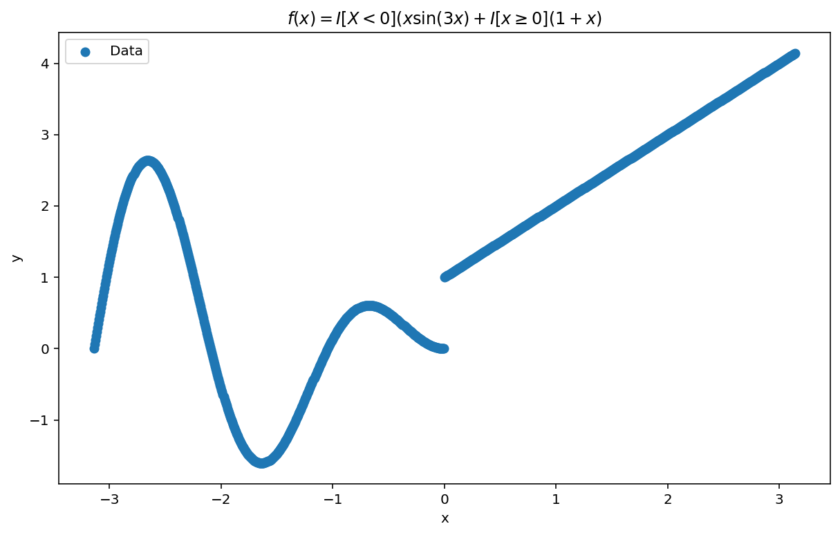
Our goal, today, will be to learn-via-example by fitting the following (highly-nonlinear) function:
$$ y = \begin{cases} x \sin(3x) & \text{if } x < 0, \\ 1 + x & \text{otherwise}. \end{cases} $$
Why this function? Well, for starters, it’s easy to visualize. Visualization allows us to get a feel for RFF and it’s capabilities and short comings. We will plot it shortly. More importantly, the function contains a number of pathologies. It isn’t continuous. It isn’t periodic across its domain. It has a non-continuous first derivative. Each of these “wrenches”, which may trip up other algorithms will showcase some of the benefits and shortcomings of RFF which is the point of this first post.
Plots
Let’s see what we are working with:
import numpy as np
import matplotlib.pyplot as plt

N_data = 1000
X = np.linspace(-np.pi, np.pi, N_data).reshape(N_data, 1)
y = [np.piecewise(x, x < 0, [x * np.sin(3 * x), 1 + x]) for x in X]

plt.figure(figsize=(10, 6))
plt.scatter(X, y, label='Data')
plt.xlabel('x')
plt.ylabel('y')
plt.title('$f(x) = I[X < 0](x \sin(3x)) + I[x\geq 0](1 + x)$')
This code is nothing special.
- We start with $N_{data}$ points
- Our input, $x$ has domain $x \in [-\pi, \pi]$.
- We set $y = \mathbb{I}[X < 0](x \sin(3x)) + \mathbb{I}[x \geq 0](1 + x)$.
$\mathbb{I}[\cdot]$ is the Iverson bracket. For simplicity, in this blog post, we will assume all the data fits in memory. It’s important to note this is not a constraint of the RFF method in general. In future blog posts, we will remove this constraint to show how RFF can be trained in a streaming fashion.
RFF is Five Lines of Code
The first amazing fact about RFF is that it is four lines of setup and five lines of “modeling” code.
There are three parameters which define the RFF approximation:
| Parameter | Rank | Description |
|---|---|---|
| $R$ | $\mathbb{R} $ | Number of “features” or “kernels” used by RFF. The more features, the better the approximation. More features comes at the cost of higher computational overhead. |
| $\gamma$ | $\mathbb{R} $ | $ \gamma $ acts as the “width” or “frequency” of the kernel approximation. Larger values of $\gamma$ favor more “local” approximations while smaller values of $ \gamma $ prefer more “global” approximations. I’ve heuristically found increasing $\gamma$ as a function of R can improve the fit at the cost of larger variance. |
| $\lambda$ | $\mathbb{R} $ | $ \lambda $ acts as a regularization term. Larger values of $ \lambda $ favor simpler functions. |
In some settings, $\gamma$ and $\lambda$ can be generalized to vectors. For this blog post, we will assume they are scalar but we may remove that restriction in future blog posts.
And now, RFF:
# Setup
np.random.seed(0)  # Set the random seed for reproducibility
R = 100            # Number of RFF samples
gamma = R / 10     # Kernel "width" parameter
llambda = 0.1      # Regularization parameter

# Here is RFF, in all it's glory...
kernel = np.random.normal(size=(R, 1))
bias = 2 * np.pi * np.random.rand(R, 1)
proj = np.cos(gamma * (X @ kernel.T) + bias.T)
weights = np.linalg.solve(proj.T @ proj + llambda * np.eye(R), proj.T @ y)
y_hat = proj @ weights

# And plot the results.
plt.plot(X, y_hat, label='RFF Approximation', linestyle='-', color = "orange", lw= 5)
plt.suptitle(f'RFF Approximation $R={R}, \gamma={gamma}, \lambda={llambda}$')
plt.legend()
plt.show()
Slowing down, let’s break each line out for explanation. $x$ is our input and $y$ is our output. Both are scalars with dimensionality $d_x = 1$ and $d_y = 1$ respectively. RFF proceeds as follows:
| Step | Shape | |
|---|---|---|
| S1: [Sample a kernel, $K$] | $K \in [R, d_x] $ | $K \sim \mathcal{N}(\mu=0,\sigma=1) $ |
| S2: [Sample a phase bias $B$] | $B \in [R, 1] $ | $B\sim 2\pi\text{Uniform}(0, 1) $ |
| S3: [Project onto random map, $P$] | $P \in [N_{data}, R] $ | $P \leftarrow \cos\left(\gamma XK^T + B^T\right) $ |
| S4: [Solve for weights, $W$] | $W \in [R, d_y] $ | Solve for $W$: $$ \left( P^TP + \lambda I(R)\right)W = P^Ty$$ |
| S5: [Predict $\hat{y}$] | $\hat{y} \in [N_{data}, d_y] $ | $\hat{y} = PW$ |
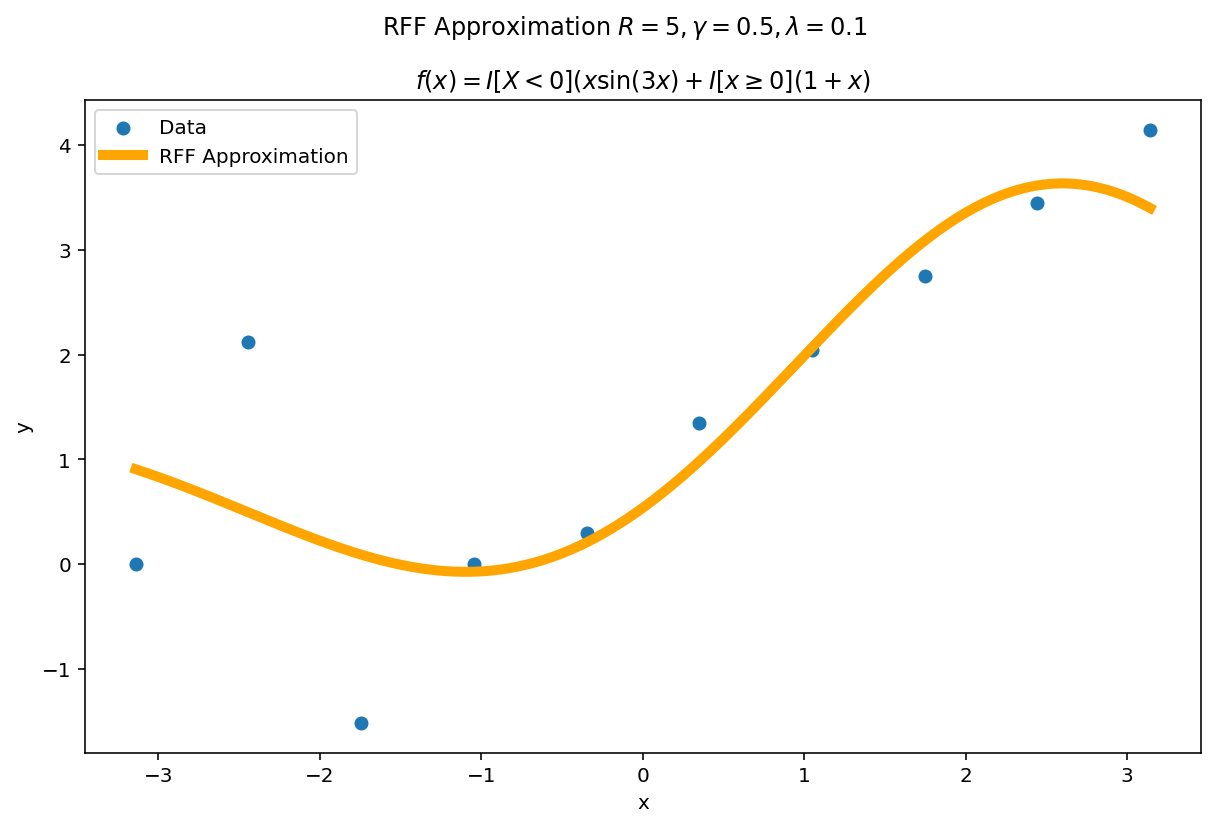
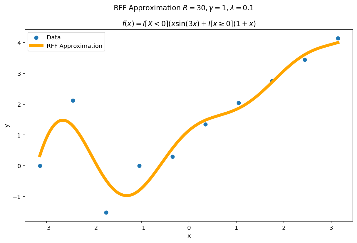
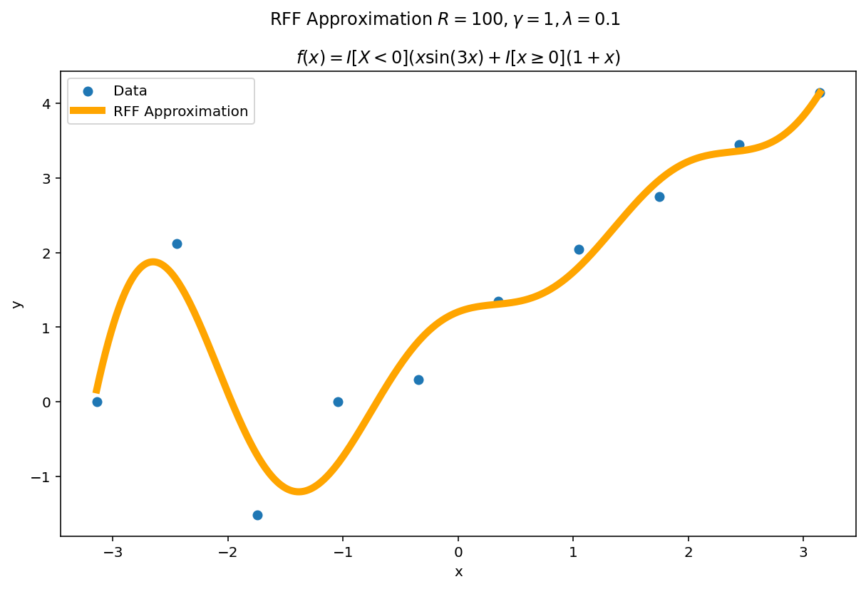
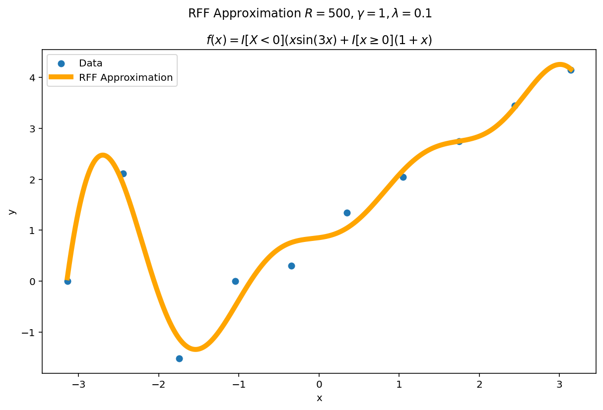
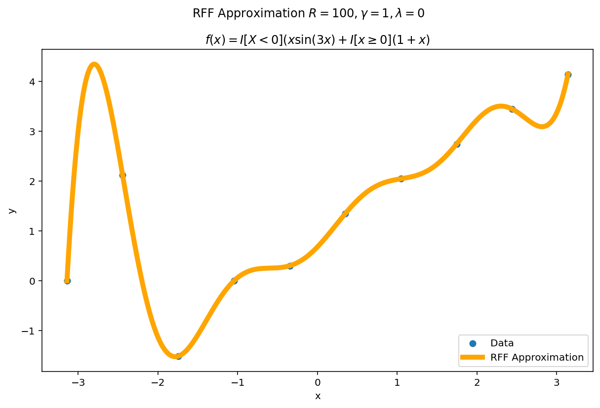
Plot the fit for various values of $R$
In RFF, the larger $R$ is, the better the approximation (on average). Let’s plot the fit of our test function for a few values of $R$. Since we have a lot of data, we will scale $\gamma$ with $R$ to allow for more flexible fits.
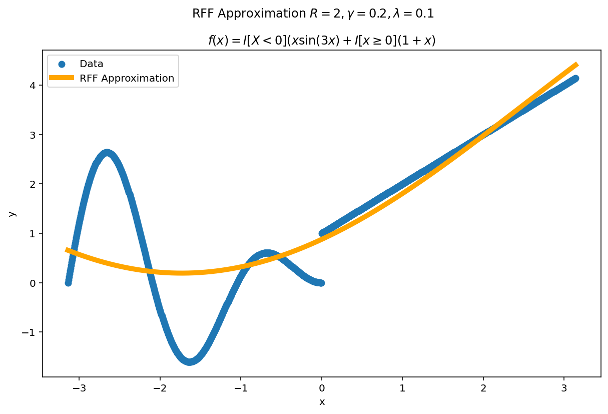
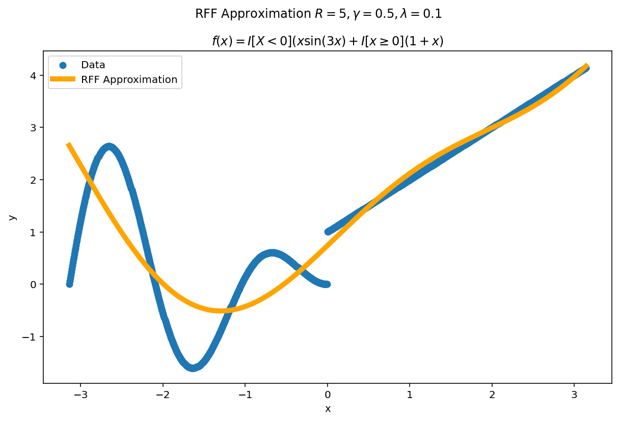
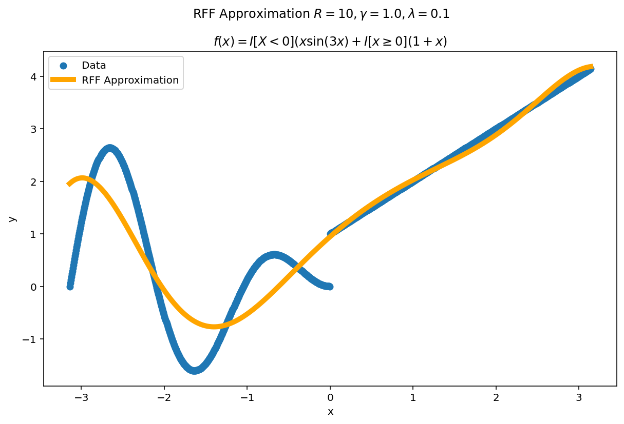
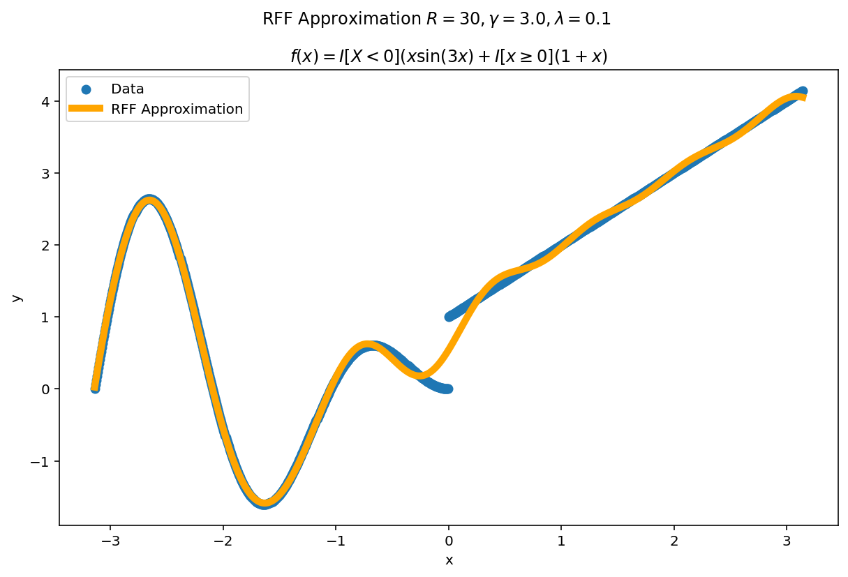
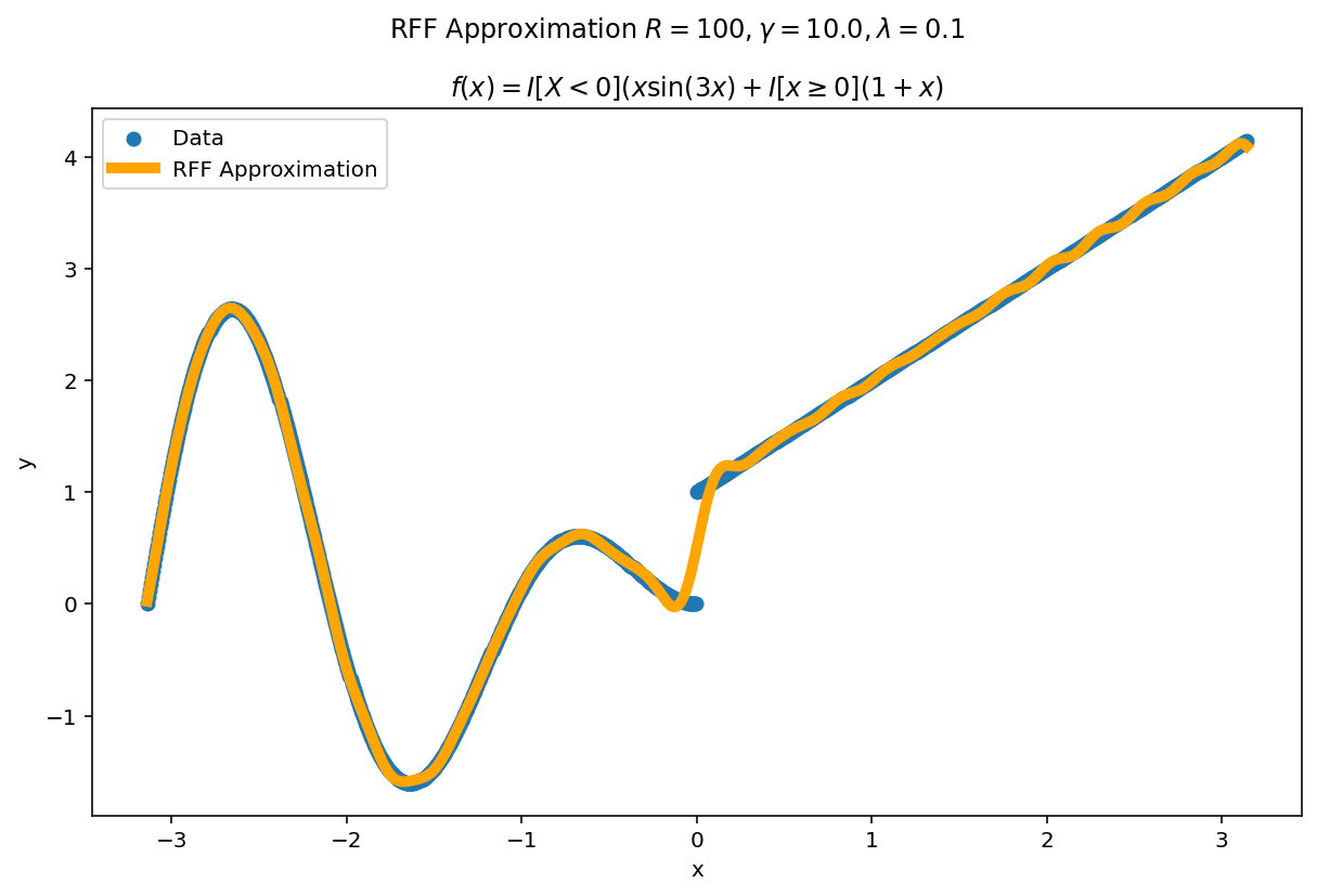
We can see a minor ringing effect in the fit, akin to Gibbs Phenomenon but the approximation fits decently well and handles the discontinuities easily.
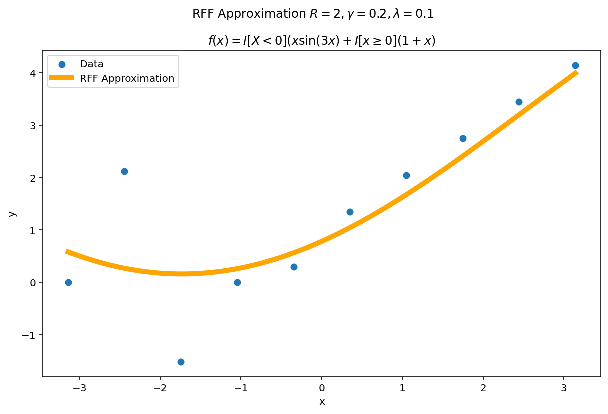
Underspecification
The function above was difficult to fit, but we had a large amount of data. What happens if we reduce the data significantly but keep the fit heavily over parameterized ? A good approximation should (a) become better with more parameters and (b) self-regularize when it is over-parameterized. This second point is important in practice: methods which fail to self-regularize can “blow-up” without other interventions. If you have ever fit a polynomial of large degree to data, you have likely experienced Runge phenomena which is one such pathology.
The second amazing fact of RFF is it has regularization built in. The parameters $\gamma$ and $\lambda$ jointly determine how flexible the fit will be in the limit. For a fixed $\gamma$ and $\lambda$ we can see this “limiting” effect by increasing $R$.
The plotting code is a slight modification from before. This time, we learn our weight matrix, $W$ using the ten training points and then use this learned weight matrix to predict for a much denser grid of plotting points. In code:
# Setup
np.random.seed(0)  # Set the random seed for reproducability
R = 30            # Number of RFF samples
gamma = R / 10
# gamma = min(1, R / 10)     # Kernel "width" parameter
# gamma = 1     # Kernel "width" parameter
llambda = 0.1      # Regularization parameter

# Here is RFF, in all it's glory...
kernel = np.random.normal(size=(R, 1))
bias = 2 * np.pi * np.random.rand(R, 1)
proj = np.cos(gamma * (X @ kernel.T) + bias.T)
weights = np.linalg.solve(proj.T @ proj + llambda * np.eye(R), proj.T @ y)

# Define plotx to be a dense grid in the domain of the function. Project
# plotx using the RFF formulation and reuse the learned weight matrix to
# estimate the RFF approximation.
plotx =  np.linspace(-np.pi, np.pi, 1000).reshape(1000, 1)
proj2 =  np.cos(gamma * (plotx @ kernel.T) + bias.T)
y_hat = proj2 @ weights

plt.plot(plotx, y_hat, label='RFF Approximation', linestyle='-', color = "orange", lw= 5)
plt.suptitle(f'RFF Approximation $R={R}, \gamma={gamma}, \lambda={llambda}$')
plt.legend()
plt.show()
Even with hundreds more interpolates than data points, the function naturally regularizes itself due to the $\gamma$ and $\lambda$ parameters.
Misspecification
What happens if $\gamma$ or $\lambda$ are misspecified?
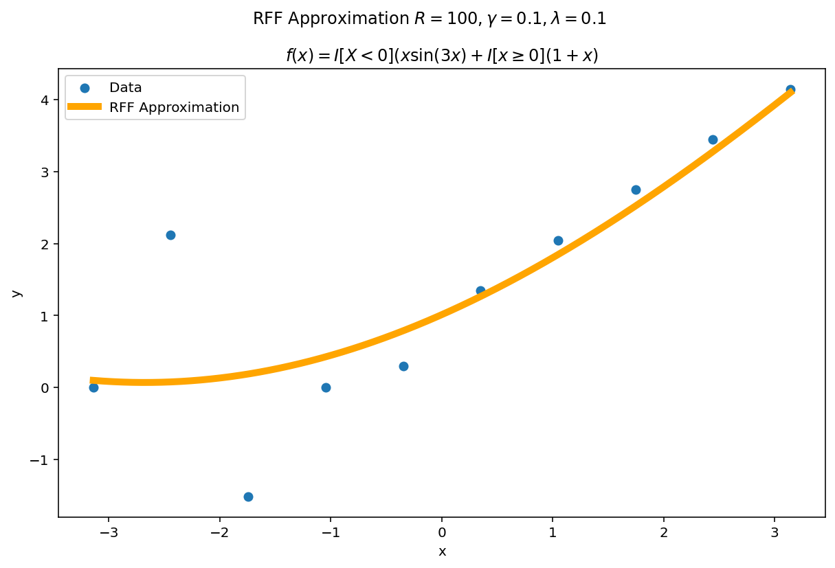
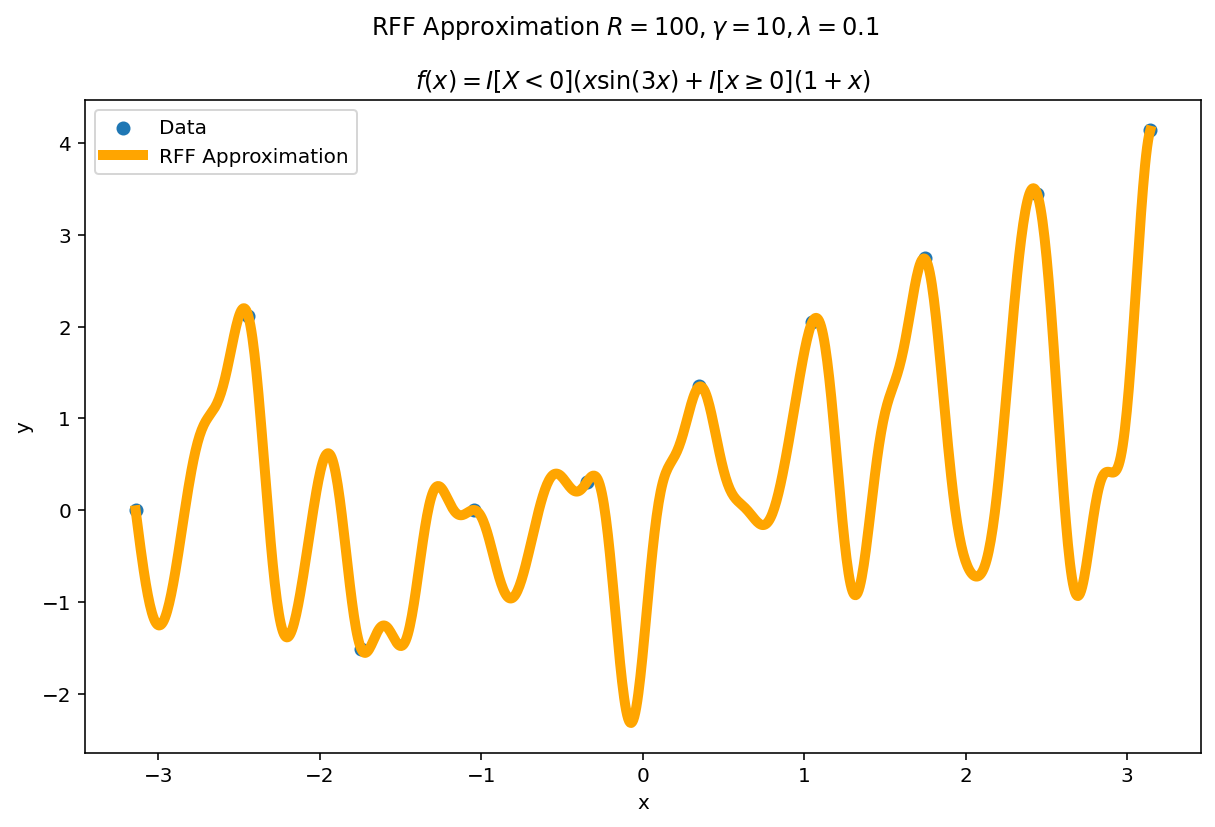
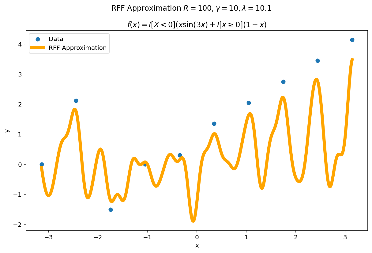
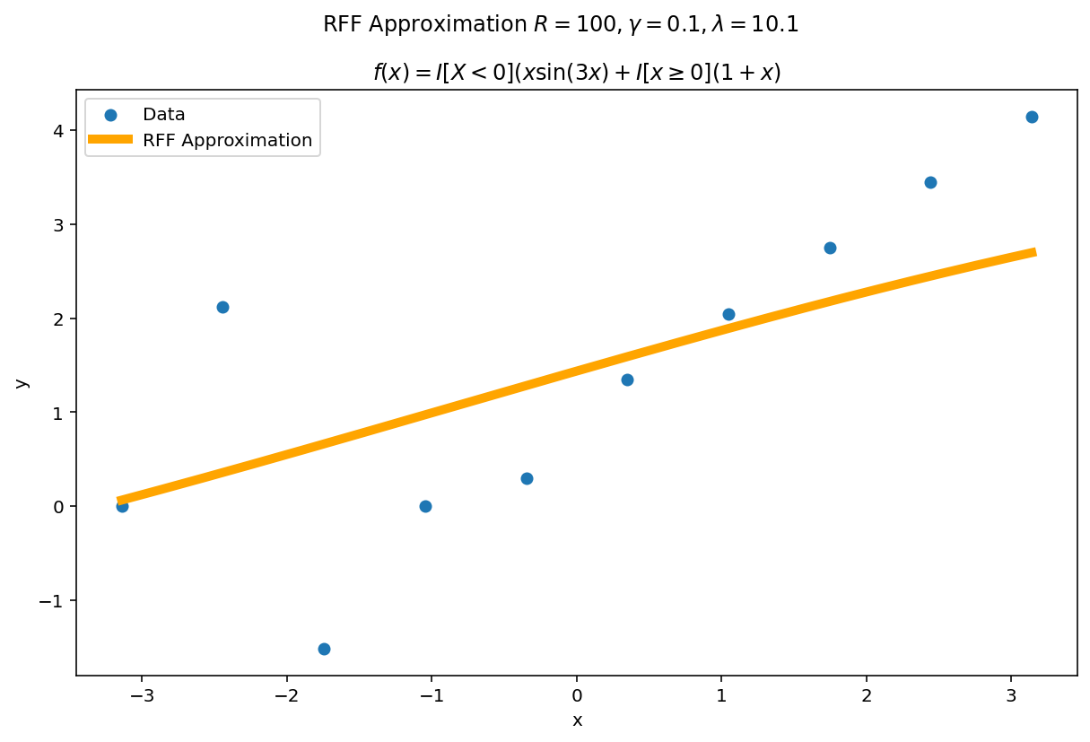
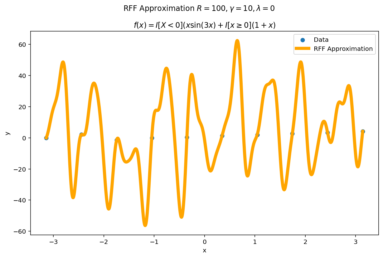
The worst fits come when $\lambda \rightarrow 0$ and $\gamma$ is larger than the intrinsic variance of the function. $\lambda$ is a regularization term, so as $\lambda \rightarrow 0$, the functional is able to fit the data perfectly at the cost of larger variance.
In practice, I typically start with somewhat larger values of $\lambda$ and somewhat smaller values of $\gamma$ and adjust them accordingly depending on the type of fit I want and how it performs on validation data.
Learning by Example: Higher Dimensions
Most analytic methods of curve fitting tend to work well in one dimensional settings but quickly become unwieldy in higher dimensions. RFF’s third amazing fact is that it works, just fine, for inputs and outputs which are multidimensional. The code changes are almost unnoticeable as well.
Function Definition
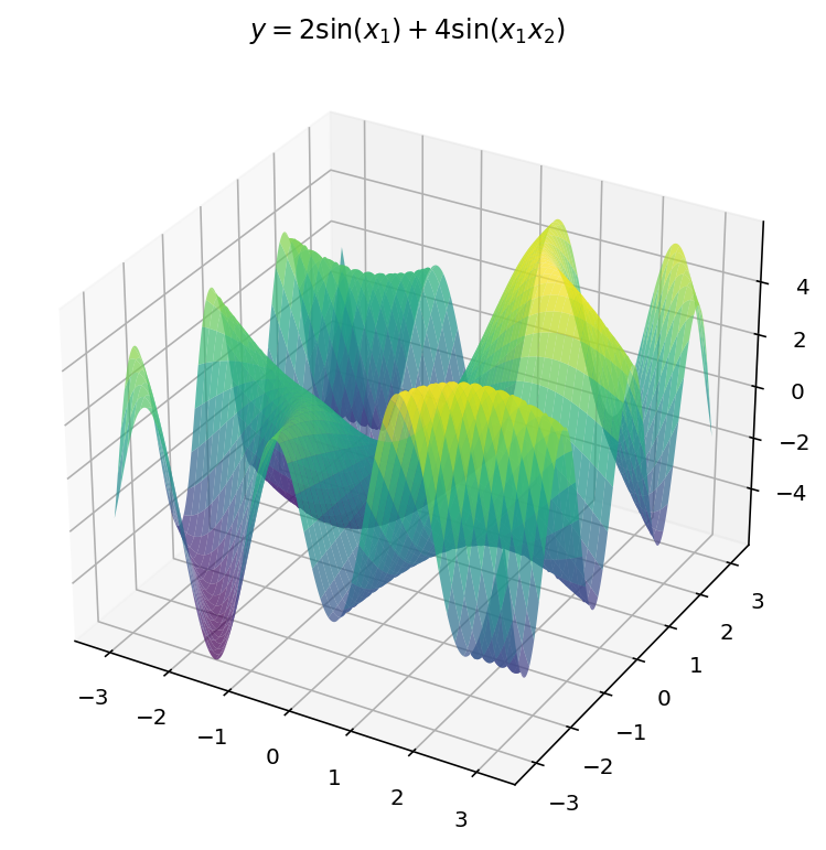
As before, we are going to learn-by-example and teach RFF to approximate the function:
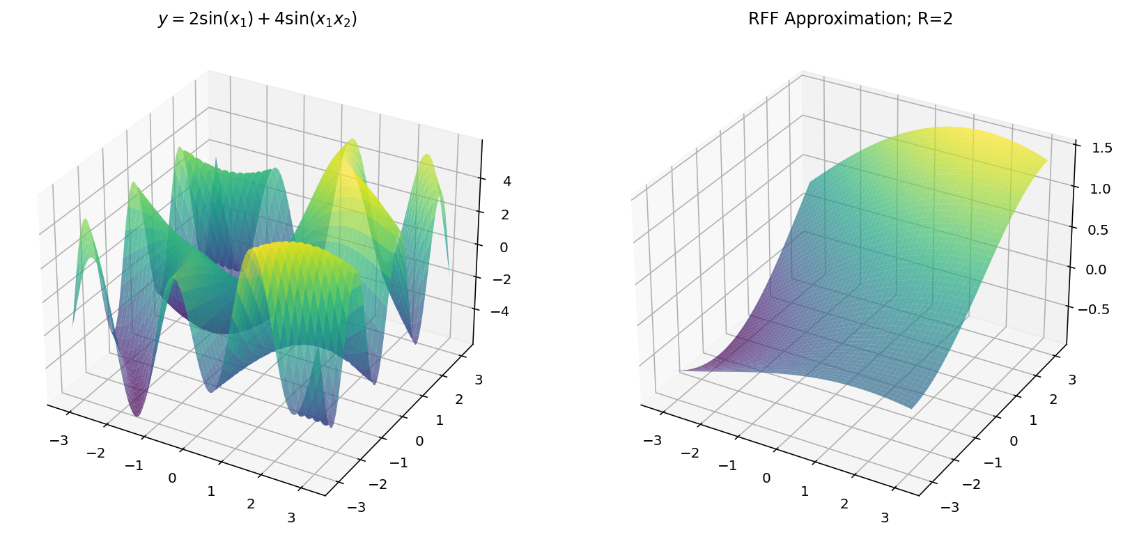
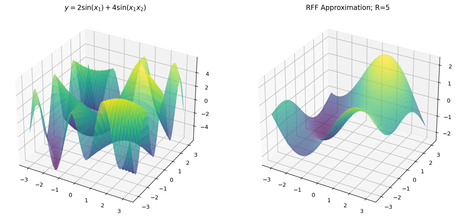
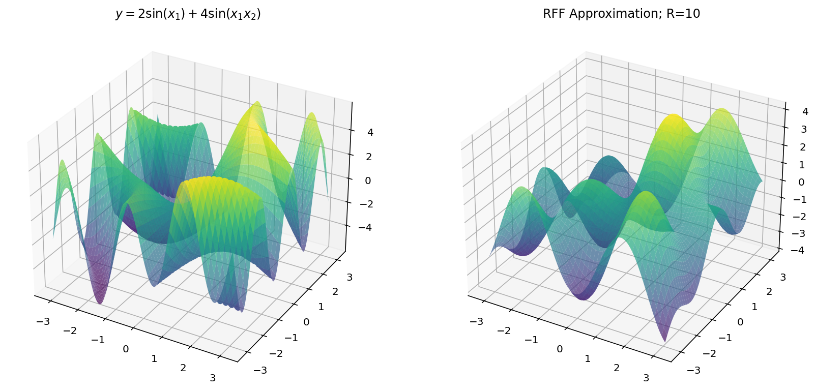
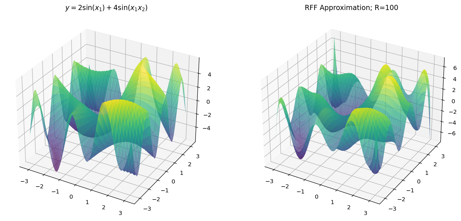
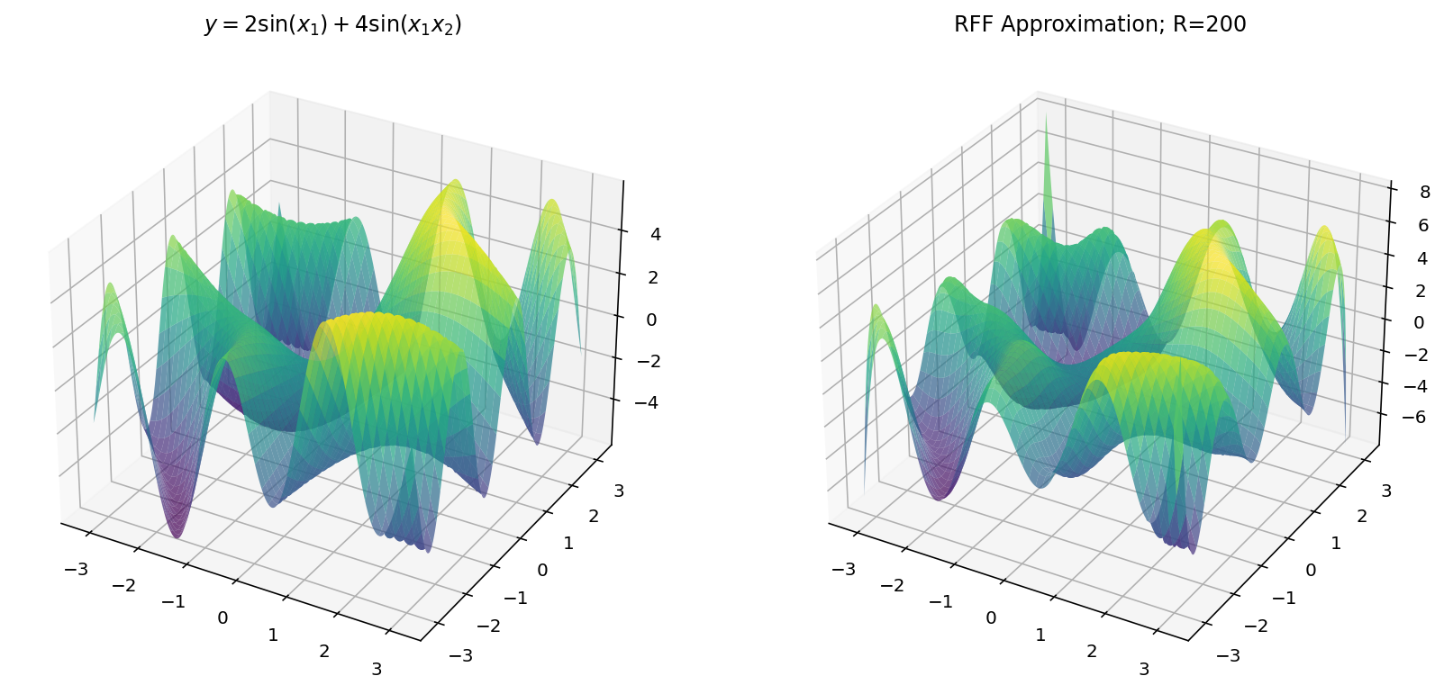
$$ y = 2 \sin(x_1) + 4 \sin(x_1x_2) $$
Unfortunately, we are limited by human biology in this exploration: with $d_x = 2$ and $d_y = 1$, we exhaust the three dimensional limitations of our eyes. Worry not, however, since we can still learn a few things in the three-dimensional setting.
Plots
The plotting code, this time, is only slightly more difficult:
import numpy as np
import matplotlib.pyplot as plt
from mpl_toolkits.mplot3d import Axes3D


# Generate multivariate data for y = 2 * sin(x1) + 4 * sin(x1 * x2)
N = 1000  # Number of data points along each axis
x1 = np.linspace(-np.pi, np.pi, N)
x2 = np.linspace(-np.pi, np.pi, N)
X1, X2 = np.meshgrid(x1, x2)
Y = 2 * np.sin(X1) + 4 * np.sin(X1 * X2)

fig = plt.figure(figsize=(14, 7))
ax = fig.add_subplot(121, projection='3d')
ax.plot_surface(X1, X2, Y, cmap='viridis', alpha=0.7)
ax.set_title('$y=2 \sin(x_1) + 4 \sin(x_1 x_2)$')
Fitting with RFF
The code for RFF is more-or-less the same as before except we have to “flatten” the $x$ and $y$ dimensions from a grid to a vector of examples.
# Setup
np.random.seed(0)  # Set the random seed for reproducability
R = 10             # Number of RFF samples
gamma = 1          # Kernel "width" parameter
llambda = 0.1      # Regularization parameter

# Flatten the inputs and outputs
X1_flat = X1.flatten().reshape(-1, 1)
X2_flat = X2.flatten().reshape(-1, 1)
X_flat = np.hstack((X1_flat, X2_flat))
Y_flat = Y.flatten()

# Random Fourier feature mapping for Gaussian kernel
kernel = np.random.normal(size=(R, 2))
bias = 2 * np.pi * np.random.rand(R, 1)
proj = np.cos(gamma * (X_flat.dot(kernel.T)) + bias.T)
weights = np.linalg.solve(
  proj.T.dot(proj) + llambda * np.eye(R),
  proj.T.dot(Y_flat),
)
y_hat = proj.dot(weights).reshape(N, N)

ax2 = fig.add_subplot(122, projection='3d')
ax2.plot_surface(X1, X2, y_hat, cmap='viridis', alpha=0.7)
ax2.set_title(f'RFF Approximation; R={R}')
plt.show()
Which, for different values of $R$ yields: